Chapter 4: Frequency Analysis and Histograms

I. Frequency Distribution Analysis

• What is Frequency Analysis?: An analysis method that counts how many data points exist for the same value or within a specific range.

• Frequency: The number of data points included in a specific value or range.

• Class: The numerical ranges used to classify data, also referred to as "Class Interval".

• Interval: The width of the class.

• Setting Classes: Classes are set between the maximum and minimum values, generally divided at equal intervals for easier comparison.

Usually, these intervals are taken at equal widths as shown below:

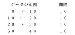
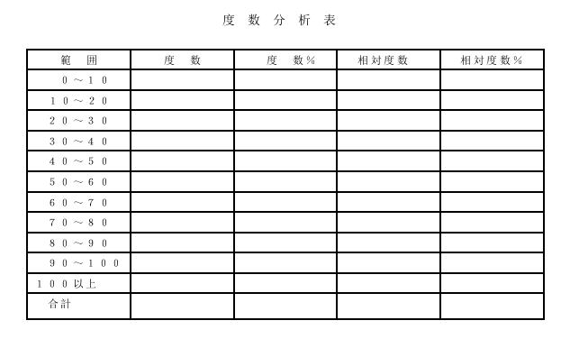
Table 1 shows a general frequency distribution table with an interval of 10.

II. Logarithmic Frequency Analysis

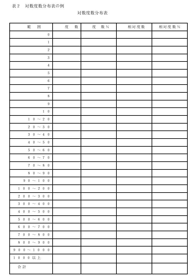
While equal intervals are common, there is also a "Logarithmic Frequency Analysis Table" that uses logarithmic scale intervals. General logarithmic intervals appear as follows:

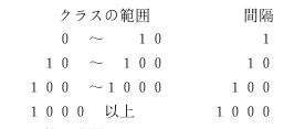
• Importance of Small-Lot Data: In EIQ analysis, small ranges like "1 to 10" are extremely important, and "Frequency 1" (single order or single shipment) holds great significance.

• Adoption of Logarithmic Intervals: When shipment volumes reach large numbers (over 10 or 100), an error of 10-20% does not significantly impact planning. Therefore, it is rational to use "Logarithmic Intervals" (widening intervals gradually) rather than equal ones.

• Segmentation from 1 to 10: For the critical volume zone of 1 to 10, detailed intervals of 1 unit (1, 2, 3...) are used.

• Utilizing "Frequency 0": By tracking items with zero shipments, you can identify "dead stock" (unmoved items) sitting in inventory.

• Standard for EIQ Analysis: In EIQ analysis, "Frequency Analysis" typically refers to analysis using these logarithmic intervals, and the term "Range" is used instead of "Interval".

III. Histogram

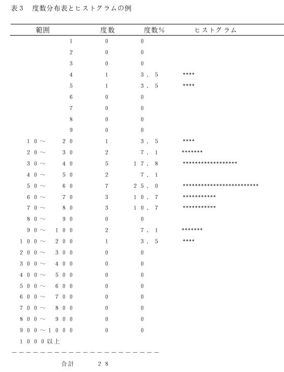
A graph representing the frequencies of a distribution table is called a histogram. Creating the graph in correspondence with the frequencies makes the data easier to read. Table 3 shows an example of a frequency table with an attached histogram.

IV. Cumulative and Relative Frequency

The sum of each frequency is called Cumulative Frequency. Values obtained by dividing frequency and cumulative frequency by the total frequency are called Relative Frequency and Cumulative Relative Frequency, respectively.

V. Frequency Analysis used in EIQ Analysis

EIQ analysis utilizes five logarithmic frequency distribution tables and histograms to understand which numerical ranges indicators are concentrated in.

1. Analysis Priorities

• Priority of EN and IK: For system planning, frequency analysis of EN (Number of items per order) and IK (Shipment frequency per item) is particularly effective, so it is recommended to start analysis with these.

2. Role of Each Indicator

• EQ Frequency Distribution (Order Quantity per Customer): Shows the range distribution of order volumes for each customer.

• EN Frequency Distribution (Items per Order): Shows the range of number of items (hits) per order for each customer.

• IQ Frequency Distribution (Shipment Quantity per Item): Shows the range distribution of shipment volumes for each product.

• IK Frequency Distribution (Shipment Frequency per Item): Shows the range of shipment frequency (order overlap) for each product.

• Q Frequency Distribution (Order Quantity per Line Item): Shows the range of order volumes for each individual line on a slip (per customer, per product).

VI. Frequency Tables and Histograms

• Structure: An analysis example covering a total of 28 samples (data points).

• Frequency and Ratio: Displays both the specific number of data points (Frequency) within each range and the composition ratio (Frequency %) relative to the total.

• Visualization: Histograms are placed alongside the numerical data, allowing users to grasp data bias and volume zones at a glance.